UNIVERSAL GEOCODING WITH A HIERARCHICAL GLOBAL
GRID
Geoffrey Dutton
Spatial Effects
20 Payson Road
Belmont MA 02478 USA
T/F 1-617-489-4524
dutton@spatial-effects.com
http://www.spatial-effects.com/
ABSTRACT
Geocoding is the process of assigning unique identifiers to
specific geographical features or locations. Following an
introduction to geocodes and issues involved in their consistency
and interoperability, the notion of constructing geocodes from
spatial coordinates is discussed, describing both planar and
spheroidal approaches. Relative advantages of the latter lead to
the conclusion that unprojected (geographical) coordinates provide
the best basis for constructing universal identifiers for many
types of spatial data. In doing so, utilizing a hierarchical
(nested) grid has many advantages, but direct use of latitudes and
longitudes is regarded as problematic because of grid cell areal
variations and degenerations. Following an introduction to
discrete global grid systems, a polyhedral approach to identifying
locations using hierarchical triangular cells which addresses
these problems is described. Its structure and encoding details
are summarized and illustrated with several worked examples. A new
algorithm for determining neighboring geocodes of a given
hierarchical location identifier is then presented. Suggestions
for incorporating semantic content into such location identifiers
are given, enabling hierarchical geocodes to describe the nature
as well as the locations of features. Requirements for spatial
indexing are briefly discussed, including handling the indexing of
both points and extended features. It is concluded that the
potential utility for global hierarchical geocoding is great, and
that technical obstacles to implementing data transfer standards
to accommodate such an approach are readily solvable, although
quite pervasive; most difficult to overcome will be a great
diversity of traditions, conventions and attitudes that affect
feature identification schemes throughout the world.
A number of systems are used to identify
parcels in the land data files currently maintained by
governmental units. While each of these identifier systems may
be adequate for a given governmental department, the existence
of several noncoordinated systems often prevents the widespread
use of the land data. Therefore, to ensure data coordination
and facilitate multiple use of data files in the cadastre, each
parcel should be identified by a unique number.
NRC (1980), p. 60.
LOCATION-BASED GEOCODING
The need to identify parcels and other geographic entities for
computer processing of geospatial data has long been recognized.
Progress in developing land information systems (LIS) and geographic
information systems (GIS) would have been impossible without
systematic attention to cataloging such information, a task generally
referred to as geocoding. Geocoding has many facets, but
chiefly is the process of assigning unique identifiers to specific
geographical features or locations. Examples of geocodes include
census codes, postal zones, parcel identifiers, benchmark
identifiers, political unit identifiers, road routes and mileposts.
Many geographic features have common names, but names are often
duplicated and can have confusing variants, and thus do not serve
well as geocodes for digital geospatial data. In general, geocodes
are assigned by fiat (usually be government agencies), and
consequently a given feature can have different identifiers when
referenced by different organizations in overlapping jurisdictions.
Even when a common nomenclature is used, dictionaries and thesauri
are required to define universes within which feature and location
identifiers are assigned, validated and interpreted. However, even
the most definitive small-area location identifiers (such as FIPS and
postal codes) are not universal, being at most national in scope.
This paper describes an approach to overcome many of these
limitations and the difficulties they engender for geoprocessing.
Zieman (1976. p 47) describes some desired properties of
geocodes:
Geocodes ... are location indices and enable the
determination of spatial or positional relationships among
entities. A location identifier should provide precise and unique
location, define both point locations and areas, be continuous
over broad areas, be suitable for statistical sampling, be
convenient for preparation and reference to various maps, relate
mathematically to the surface of the earth, and, therefore,
utilize rectangular coordinates. (emphasis added).
Zieman's perspective is pursued in this paper, which, however,
rejects the contention that rectangular coordinates (Cartesian
projections) are necessary for geocoding. As has been advocated for
many years (Moyer and Fisher 1973) a geocode can be derived from the
coordinates of a geographic point on or in a feature by hashing,
interleaving or other methods; this has been proposed for creating
parcel identifiers in land information systems. However, unless based
on latitudes and longitudes or globally, systematically constructed
using standardized projections and zones, such geocodes may not be
unique. If they encode projected coordinates, knowledge of projection
parameters may be needed in order to relate such geocodes to other
objects and locations. However, geocodes based on locations have many
potential advantages, if well implemented:
- They can be made to be globally unique
- They can be hierarchical, hence scale-specific
- They can support spatial indexing for data retrieval
- Their parsing need not depend on contextual knowledge, only
algorithms.
Geocodes derived from spherical coordinates based on a geocentric
ellipsoidal datum in principle can be made to be uniform and unique
across the globe. The reference grid can have any topology, as long
as it is reasonably regular and complete. If the grid permits
nesting, a spatial hierarchy can be defined within it that enables
geocoding to specific resolutions, virtually without limit. This also
helps them to accommodate various sizes of features. Also, because a
geocode can be mapped to a definite area on the earth's surface, it
can be used to sort stored spatial observations to index them for
storage and retrieval. The final point means that codebooks and
metadata (such as enumerate FIPS identifiers) may not be needed to
describe the universe to which a geocode belongs (e.g., the counties
of the U.S.). However, this assumes that the data user already knows
what that universe is. This too can be conveyed using qualified
(metadata-enriched) hierarchical geocodes, as is described
subsequently.
The most obvious and established way to grid a planet
(hierarchically or not) is to use quadrilaterals defined by
intersecting meridians and parallels. While there is no difficulty in
establishing such pseudo-rectangular grids, results are sub-optimal
in several respects:
- Accuracy varies, as a degree of longitude varies by the cosine
of latitude from about 111 km at the equator to zero at the
poles
- Consequently, the shapes and sizes of lat-lon quadrilaterals
vary considerably, narrowing at higher latitudes
- The quadrilaterals degenerate to triangles at the poles
Although area inequalities can be corrected by using appropriately
projected coordinates (Chen and Tobler 1986), this usually creates
major shape distortions in higher latitudes by tearing apart and
stretching the globe. A triangular mesh, such as is described
below, avoids gross distortions of size and shape (but never
completely eliminates them) and has no singular points (e.g., North
and South poles).
|
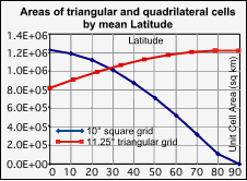
Changes in area occupied by geographic quadrilaterals can
be significant. Figure 1 shows the degeneration of area with
latitude characteristic of square grids (using a 10°
grid here), shown by the blue curve. A triangular grid of
similar resolution (11.25°), shown as the red curve,
has greater cell area closer to the poles, but the overall
change in size is considerably less. Moving between 0°
and 80°, quadrilateral grid cell area decreases by a
factor of 12, while triangular grid cell area increases by a
factor of 1.5. Thus variation in cell area is more than 800%
greater for quadrilaterals than for triangles. The
particular triangular grid used in this comparison is the
Octahedral Quaternary Triangular Mesh, described below.
Other triangulations of the globe are possible which exhibit
even less areal variation (e.g., Lee and Samet 1998), but
are more complicated to construct and utilize. It should be
underscored that global tessellations can achieve complete
areal equality only when performed on equal-area
planar projections.
|
|
|
|
Figure 1: Comparison of mesh cell areas
|
Global Hierarchical Location Encoding
Various approaches have been developed for tessellating a planet,
most of which are designed to serve a specific purpose. One
well-known effort for indexing geospatial data (Chen and Tobler 1986)
divides a projected world map (in authalic coordinates) into
hierarchically contained square cells using quadtree area indexing
(Samet 1990). This yields easily-manipulated facets of equal area
(thus its plot in figure 1 would be a horizontal line), but as
mentioned above manifests considerable shape distortions, and a
singularity at each pole. Using authalic or any other rectangular
coordinate system to organize a hierarchical rectangular grid has
these and other drawbacks, as various authors have pointed out
(Goodchild and Shirin 1991; Dutton 1998; Sahr and White 1998), and
will not be further considered below.
A general term for regular subdivision of a planet is a
discrete global grid systems (DGGS). Sahr and White (1998)
define a DGGS as a series of non-overlapping areal cells that
completely partition a sphere topological equivalent. The cells may
be triangles, quadrilaterals, hexagons or other simple polygons, and
may include just one or more than one type of polygon. The series of
grids that define a given DGGS can have hierarchical relations
that may (like conventional quadtrees) or may not (like hexagon
grids) be completely nested. Most DDGS implementations root the grids
in one of the five platonic polyhedra (tetrahedron, hexahedron,
octahedron, dodecahedron, icosahedorn) that is oriented to the planet
in a specified way. Edges of cells at levels below the root
polyhedron may follow great circles or not, and the shapes and areas
of these cells will vary in certain well-defined ways according to
the form of subdivision (White et. al. 1992). The irregularities are
inescapable (no polyhedron beyond 20 faces can have completely
uniform subdivisions) but can be engineered to minimize certain
distortions at the expense of other less important ones.
Given the choices available for root polyhedra, cell geometries,
grid topologies and cell hierarchies, a great many DGGSs are
possible, far too many to discuss here (but see overviews in White et
al. 1992 and Sahr and White 1998). There is no "best" DGGS, just as
there is no "best" map projection; one's choice depends on the needs
of the application. Thus different DGGSs tend to be advanced for
spatial indexing than for discrete simulations or for environmental
sampling, to give some examples. Sahr and White (1998) give four
design choices that creators of DGGSs based on platonic polyhedra
must always consider:
- The base platonic solid
- The orientation of the base platonic solid relative to the
planet
- The hierarchical spatial partitioning method defined
symetrically on the faces of the base platonic solid
- The transformations between each face and the corresponding
spherical surface.
Note that even though there are only five platonic solids, they
can be truncated and intersected to create semi-regular base
polyhedra. For example, an cube can be truncated to become a
cubeoctahedron (six squares and eight triangles), an icosahedron
truncated to create a solid with 20 hexagons and 12 pentagons, and a
cube and octahedron can be intersected to form a rhombic dodecahedron
(12 rhombi). Given any such base shape, it must be given a well
defined orientation to the planet, which can place vertices, edges or
face centers at the poles, or similarly along the equator; the more
faces the base shape has, the more orientation possibilities exist. A
method of subdivision then needs to be specified that allows the
polygons on the base shape to be subdivided, typically into
triangles, rhombi and/or hexagons; the greater the diversity of
sub-facets, the more complex will be the algorithms that accomplish
this. Finally, rules to map sub-facet vertices and edges to the
sphere or spheroid need to be established. Edges may follow great
circles, parallels or other lines; usually these are explicit
transformations, but in some designs (including the one described
below) at least some edges may be recursively defined and not
correspond to any simple geometric curve.
As mentioned above, most DGGSs are constructed for a specific
purpose, such as environmental data sampling, spatial process
simulation, geospatial data indexing, planetary visualization
modeling or geographic location coding. No single design serves all
purposes equally well, and thus a variety of DGGSs have been
proposed, each thought to be especially appropriate to some
envisioned application. Geographic information science is far from
yielding theories capable of specifying how to optimize DGGS design
choices, and to obtain one much experimentation must take place.
There is also currently a lack of methods to transform cells from a
given DGGS into a different one, because in almost all cases a 1:1
mapping between their elemental facets does not exist. If we
concentrate just on applications of location encoding, as we will for
the remainder of this article, the non-unique mapping between
elements in different DGGS implies that a facet identifying a given
area in one system may map to several in another system, usually
portions of several, unless the object being identified can be
regarded as a dimensionless point. However, even when an entity is
modeled as covering an area, it still can be characterized by some
interior point for identification purposes. Dimensional collapse
simplifies the name translation problem to finding a 1:1 mapping
between DGGS elements in different grids, even though such operations
can involve tricky geometric computations and possibly some arbitrary
assumptions or rules.
LOCATION CODING USING A QUATERNARY TRIANGULAR MESH
The specific hierarchical location reference system being proposed
here for global geocoding is called quaternary triangular mesh (QTM).
This model has evolved from one designed for digital elevation
modeling (Dutton 1984), subsequently recast into its current form to
facilitate global spatial indexing (Dutton 1989; Goodchild, Shirin
and Dutton 1991), positional data quality management (Dutton 1990,
1992, 1996), terrain modleing (Lugo and Clarke 1995) and map
generalization (Dutton and Buttenfield 1993; Dutton 1999). A Ph.D.
dissertation (Dutton (1998) provides an overview of QTM's
development, properties and application to map generalization. To
create a QTM, an octahedron is aligned to the earth with its
six vertices at cardinal points, fitted to an ellipsoid describing a
global datum such as WGS 84. The process of hierarchically
identifying locations begins by dividing any of its eight faces at
edge midpoints to define four child triangular facets, as
figure 2 illustrates. This simply requires computing arithmentic
averages of the latitudes and longitudes of vertices. Note that all
such first-level (and higher level) facets -- although identical on
the octahedron -- vary slightly in size and shape when the new
vertices are projected to the spheroidal or geoidal surface (local
relief, were it to be encoded on top of this, would further distort
facets).1
Subdivision may be recursively repeated as many times as are needed
to locate something on the ground: 10 levels of subdivision produce
facets about 10 km wide, 20 levels yield 10 m across and 30 levels
yield 1 cm facets. By consistently numbering the original eight faces
and their children, every facet -- no matter how small -- will have a
unique integer identifier (a base8 digit followed by some number of
base4 digits). Longer QTM identifiers (QTMIDs) are more
precise than shorter ones, as resolution improves by powers of two. A
set of QTMIDs thus is equivalent to a linear quadtree (Gargantini
1982), a set of leaf node identifiers that specify the tree's
branching structure by implication only. Interior nodes are not
needed, as the only information needed to decode any given QTMID into
coordinates that define that facet (or define a representative point
for it) are:
- The alignment of the octahedron to the planet
- The ordering of the octahedron's eight faces
- The algorithm used to assign child facet numbers
- The number of significant digits in the given geocode
- A reference ellipsoid for the region, if required
Given these parameters and an algorithm, precise geographic
coordinates of its defining triangle can be recovered from any QTMID.
If the geocode represents a very small feature, it may also alias
other small ones nearby if the depth of encoding is not sufficient to
distinguish their locations. This could be problematic if data
density varies considerably, especially when a fixed level of QTM
resolution is used to geocode a large population of features. Of the
above five elements, the third one is potentially most confusing.
Several schemes have been proposed for numbering QTM facets, each of
which produces different geocodes for a given location (Fekete 1990;
Otoo and Zhu 1993; Lugo and Clarke 1995). However, all these encoding
implementations traverse identical sets of triangular facets, because
all align the octahedron in the same fashion (but note that while
Fekete's numbering system is congruent with the author's, his trees
are rooted in an icosahedron). Therefore, even if different
algorithms are used to encode a given feature, a direct 1:1 mapping
between the resulting geocodes exists (Fekete's model excepted, again
because of its different base solid).
|
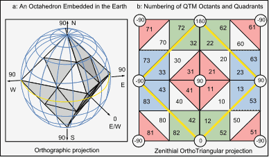
Figure 2 illustrates the basic structure of QTM. In 2a,
an octahedron is centered on the earth's center of mass and
aligned with cardinal points; its first-level facets are
shown prior to being pushed toward the surface of the
planet. In 2b, the first-level facets are shown in a global
projection with the North Pole in the center and the South
Pole at the corners; the yellow diamond is the Equator.
Geocodes (QTMIDs) are shown for each of the initial 32
facets; the first digit is the octahedral face ID (octant),
and the second digit is the facet ID within an octant. All
facets with the same last digit are given an identical
color. Note that facets whose IDs end in 0 are centrally
located; subsequent subdivisions preserve this property, but
permute the cyclic ordering of facets ending with 1, 2 and
3. Numbering properties are explained further
below.
|
|
|
|
Figure 2: Structure of Octahedral Quaternary
Triangular Mesh
|
|
The figure of the QTM grid on the globe is displayed in
figure 3 (black lines), where it is overlaid on a 22.5°
geographic grid (light blue lines). Although neither grid is
totally uniform, the geographic grid can be seen to have
more variability, as figure 1 describes quantitatively. Note
that both grids follow parallels (but only the cardinal
meridians are common to both). The spacing of the parallels
of the QTM grid, however, is defined by the relation 90 /
2L, where L is the QTM level of detail (from 1 to
c. 30), as is spacing of the longitudes that define corner
points of QTM facets.
Note that the shapes of facets vary from equilateral
spherical triangles at the centers of octahedral faces to
right spherical triangles at their corners. However, locally
-- especially at higher levels of detail -- facet shape is
not especially variable. This means that for locations
within 1,000 km or less of one another facets are relatively
uniform.
|

|
|
|
Figure 3: The QTM Grid and the Geographic Grid
(Orthographic Projection)
|
QTM Geocoding: Example 1
Because four children develop from each parent facet, the
structure is a quadtree ("quaternary"). A QTMID is thus a base4
number preceded by a base8 digit, and each base4 digit requires two
bits of memory to encode. Here is a QTMID from eastern North America,
encoding the position 42° 23' N, 71° 10' W to
about 10 km resolution:
40223012232 (QID1)
Octant 4 (the first digit) also covers the westernmost portions of
Europe and Africa, southern Central America, northern South America
and the Caribbean (most of Mexico, the U.S. and Canada are in octant
3). The above geocode has 10 quaternary digits; at this level of
detail, QTM facet edges are about 10 km across and facets occupy 61
sqkm of area on the average. If we assign 4 bits to store the octant
ID and 2 bits for each quaternary digit, this geocode could be stored
or transmitted using 24 bits. By converting the identifier to binary
notation, this is clear:
0100 00 10 10 11 00 01 10 10 11 10 (QID1a)
Because both binary and quaternary numbers are unfamiliar and my
have a lot of digits, it makes sense to express such geocodes in a
more compact way. We could express a QTMID using decimal digits, but
hexadecimal notation makes more sense and is more compact:
42B1AE (QID1b)
While not many people are familiar with hex numbers, they are used
to dealing with postcodes; a hex-formatted QTMID (HQTMID)
looks quite a lot like postal codes used in Canada and the U.K. The
resemblance, while superficial, may help to make QTMIDs less
perplexing. Postcodes, while they are logically assigned and
generally represent some type of spatial ordering, are not directly
convertible to geographic locations, as are QTMIDs.
QTMID 40223012232 (42B1AE) includes most of the town
of Belmont MA, USA, where the author lives. To further specify the
particular parcel his house occupies requires roughly 10 m precision.
This necessitates adding 10 more quaternary digits:
402230122320130032201 (QID2)
Producing this ID presumes the ability to locate a representative
point in the parcel to within 10 meters, or about 0.3 arc-seconds.
This is certainly possible with civilian GPS and remote sensing
technologies. The binary version is thus:
0100 00 10 10 11 00 01 10 10 11 10 00 01 11 00 00 11 10 10 00 01 (QID2a)
Finally, the hexadecimal version of the parcel code is:
42B1AE1B3A1 (QID2b)
This geocode locates the parcel at 20-22 Payson Road (a duplex
condominium on one lot), and can be coded using 44 bits. Postcode
aficionados may observe that 11 hex digits take up more storage space
than the 9 decimal digits used by the U.S. ZIP+4 postal codes, which
are sufficient to geocode any address in that country. In response,
it should be noted that:
- The geographic universe of ZIP codes is a minority subset of
the whole planet's addresses
- ZIP codes encode addresses along roads, thus are inherently
1-dimensional
- QTMIDs encode all areas of land and water uniformly,
regardless of human occupancy
It therefore should not come as a surprise that QTMIDs require
more storage than ZIP+4 geocodes to represent a parcel. This should
be apparent from the illustration of QTM referencing for the above
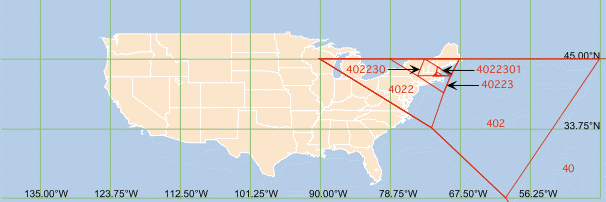
address 40223012232 given in figure 4. In it, QTM facet
boundaries are shown in red, and the largest one shown (part of facet
40, which is mainly occupied by the Atlantic ocean) extends from
0°W to 90°W at 45°N, and has a bottom apex (not shown)
at 45°W, 0°N, near to the coast of Brazil. The
equicylindric projection used maintains straight parallels (one edge
of every QTM facet is on a parallel), but the shapes of land masses
and facets are distorted, the latter due to lack of intermediate
points along facet edges (the edges that do not follow parallels are
piecewise continuous curves that are neither small nor great
circles).
|
|
Figure 4: Hierarchical Geocoding for QTMID
402230112232 Starting at QTM Facet 40, equicylindric
projection
|
QTM Geocoding: Example 2
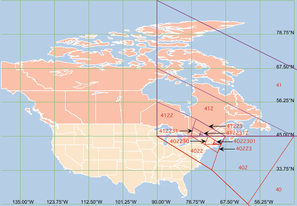
Here is another North American QTM geocode, in Canada:
41223123202 (QID3)
This facet includes most of Ottawa, Ontario and Hull, Quebec.
Ottawa is about 500 km from Belmont, Massachusetts. This is reflected
by the fact that their QTMIDs differ by only one digit of the first
five in their respective addresses (40223 v. 41223).
Because facet 40 abuts facet 41 (by definition of the
numbering scheme, facets ending in zero are always central ones of a
set of four children), the two hierarchies begin as neighbors. In
fact they occupy neighboring facets until QTM level 5 is reached.
This can be seen in figure 5, which shows both QTM sequences together
(the Ottawa hierarchy is shown in magenta).
The binary version of QTMID 41223123202 is:
0100 01 10 10 11 01 10 11 10 00 10 (QID3a)
Its hexadecimal encoding is:
46B6E2 (QID3b)
|
|
|
Figure 5: Hierarchical Geocoding for QTMID
41223123202 starting at QTM Facet 41, equicylindric
projection
|
The geocode for Ottawa-Hull is based on the position given for the
Ottawa Geomagnetic Observatory in its web pages: 45.403' N,
75.552' W. Assuming all digits are significant for this position,
its precision indicates an accuracy of about 100 m (presumably the
Observatory has a better estimate if it is part of a geodetic
network). If it sits on a large enough parcel, 100 m of error would
be small enough to uniquely locate the observatory, and would require
17 QTM levels of detail (c. 75 m resolution). So, to fully geocode
the location 45.403°N, 75.552°W, we add seven more digits
to the QTMID:
412231232021330000 (QID4)
Note that all the trailing zeros are significant. Furthermore,
because a facet numbered zero is always the middle one at any level,
the actual location of the facet centroid does not change for the
four highest levels; facet 412231232021330000 is precisely in
the middle of facet 41223123202133, but just one-sixteenth as
wide. Centroids of both facets would evaluate to the same latitude
and longitude, but the longer QTMID documents considerably higher
accuracy.
Construction of QTM Identifiers
|
Numbering of QTM facets may seem non-intuitive but it is
logical and has three-axis symmetry. As figure 5 above
illustrates, all neighboring facets of the same level of
detail have geocodes that differ by exactly one digit. This
is true even if they fall in neighboring octants (in which
case, the first digit will differ). Figure 6 illustrates the
structure of the numbering system, which is entirely based
on single-digit basis numbers assigned to the
octahedron's vertices and facets. This is organized as
follows:
- The octahedral facets all have basis number 0 (not to
be confused with their octant IDs which range from
1 to 8)
- The North and South Poles have basis number 1
- Octa vertices where the Equator crosses the 0th and
180th meridians have basis number 2
- Octa vertices where the Equator crosses the 90th and
270th meridians have basis number 3
When a facet is subdivided into four, a digit {0|1|2|3}
is appended to its QTMID
|
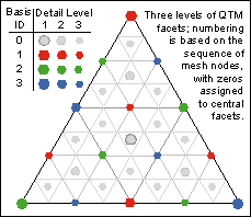
|
|
depending on which child facet is being occupied.
|
Figure 6: How QTMIDs are assigned
|
The central child facet inherits basis number 0 in all cases. The
other three children are assigned the basis number of the parent
vertex they touch. New vertices appear at the midpoints of facet
edges (these vertices have latitudes and longitudes that are the
average of those of the parent's vertices which define the edges).
The basis numbers assigned to the midpoint vertices plus those of the
endpoints always total 6. Therefore:
- Basis 1 vertices appear at the centers of edges
connecting basis 2 and basis 3 vertices
- Basis 2 vertices appear at the centers of edges
connecting basis 1 and basis 3 vertices
- Basis 3 vertices appear at the centers of edges
connecting basis 1 and basis 2 vertices
This algorithm creates the pattern of vertices shown in figure 6.
The diagram displays the prototype numbering for QTM Octants 1, 3, 6
and 8 (the remaining Octants differ only in that they interchange the
initial basis 2 and 3 "baseline" vertices. Coloring the unmarked
vertices (level 4) is left as an exercise for the reader.
Finding Neighboring QTM Facets
To be able to traverse any QTM-based data structure, one must have
a way to identify the neighbors of a given facet (the three facets
which border it, ignoring neighbors which meet at a vertex). A very
fast (constant-time) way to do this was presented by Lee and Samet
(1998); however, this study modeled the globe as an icosahedron
(having 20 rather than 8 faces) and numbered facets differently than
as described above; thus this low-level method cannot be used for
O-QTM without revision. Here we describe a linear-time (with respect
to the number of QTM levels of the QTMID being analyzed) traversal
algorithm that is even simpler than the one given by Lee and Samet;
because the algorithm does not use logical bit operations, it should
be easier for the reader to understand. A C-language implementation
of this algorithm, getQTMneighbors(), presented here for the
first time, is listed below. Given a QTMID encoded as an array of
integers (with octant ID in position 0) and its number of QTM levels
(or some lesser level at which neighbors are to be identified), it
computes and returns three arrays of integers respectively
representing: (a) the QTMID of the facet to the north or south of the
given one; (b) the QTMID of facet to the east; and (c) the QTMID of
the facet to the west. The function returns TRUE if the given facet's
apex points north or FALSE if it points south, in order to establish
the direction of the vertical neighbor.
int      getQTMneighbors(int q[], int levs, int q_v[], int q_e[], int q_w[])
/*
     Computes edge neighbor IDs of a given QTM facet. Returns N-S logical orientation of q.
     Parameters:
       q[]:   Given QTM facet QTMID
       levs:  Number of levels of q[] (array length-1)
       q_v[]: Returned QTMID of north/south neighbor
       q_e[]: Returned QTMID of east neighbor
       q_w[]: Returned QTMID of west neighbor
     copyright © 1999, 2000 by Geoffrey Dutton. All rights reserved.
*/
{
int      oct, d, i, upright, edge_id[3], edge_lev[3], node_id[3];

oct = q[0];
edge_id[1] = 1 + (oct+8) % 4 + (4*(oct / 5));
edge_id[2] = 1 + (oct+6) % 4 + (4*(oct / 5));
if (oct < 5) edge_id[0] = oct + 4;
else edge_id[0] = oct - 4;
upright = oct < 5;                                 //orientation: TRUE if facet points to North
node_id[0] = 1;
if ((oct % 2) == 0) {
    node_id[2] = 2; node_id[1] = 3;
} else {
    node_id[1] = 2; node_id[2] = 3;
}
edge_lev[0] = edge_lev[1] = edge_lev[2] = 0;       //edge neighbors now defined at QTM level 0

for (i=1; i <= levs; i++) {                        //visit every QTM level starting from 1
    d = q[i];
    if (d == 0) {                                  //central quad: all neighbors change IDs
        upright = !upright;                        //north & south flip in central quad
        iswap(&node_id[1], &node_id[2]);           //interchange east & west node numbers
        edge_lev[0] = edge_lev[1] = edge_lev[2] = i;
        edge_id[0] = node_id[0];                   //store the neighbor IDs across the 3 edges
        edge_id[1] = node_id[1];
        edge_id[2] = node_id[2];
    } else if (d == node_id[0]) {                  //vert quad: only vert neighbor changes ID
        iswap(&node_id[1], &node_id[2]);           //interchange east & west node numbers
        edge_id[0] = 0;                            //Neighbor across vert edge is central
        edge_lev[0] = i;
    } else if (d == node_id[1]) {                  //east quad: only west neighbor changes ID
        iswap(&node_id[0], &node_id[2]);           //interchange vert & west node numbers
        edge_id[1] = 0;                            //Neighbor across west edge is central
        edge_lev[1] = i;
    } else {                                       //west quad: only east neighbor changes ID
        iswap(&node_id[0], &node_id[1]);           //interchange vert & east node numbers
        edge_id[2] = 0;                            //Neighbor across east edge is central
        edge_lev[2] = i;
    }
}
for (i=0; i <= levs; i++) {                        //copy q to all 3 output IDs;
    q_v[i] = q_e[i] = q_w[i] = q[i];               //one digit of each will be modified
}
i = edge_lev[0];                                   //level at which vert edge last changed
q_v[i] = edge_id[0];
i = edge_lev[1];                                   //level at which east edge last changed
q_e[i] = edge_id[1];
i = edge_lev[2];                                   //level at which west edge last changed
q_w[i] = edge_id[2];
return upright;                                    //return the orientation of given facet q
}
|
The comments included above explain the logic of the procedure,
which exploits the following structural properties:
- All three neighbors of a given facet have QTMIDs that differ
from its own in one digit only (however, the converse is not
always true)
- There is one neighbor to the east, to the west and to the
north or south
- A neighbor's QTMID only changes when a new edge is
established
- When the final digit in a QTMID is 0, the child facet is
central and 3 new edges are created
- When the final digit in a QTMID is 1, 2 or 3, one new edge is
created (always interior)
- The permutation of vertex basis numbers controls the QTMID
digits assigned to facets and their edge neighbors
- North-south (vertical) facet relationships interchange when a
central (0) facet is entered, not otherwise
Note that the QTMID arguments could be 64-bit integers rather than
arrays, which would have to be parsed using bit manipulations. While
this could easily be done, including such operations would obscure
the essence of the method, and thus the implementation details have
not been described.
Incorporating Semantic Content Into Geocodes
A QTMID -- or any location-based geocode -- describes where
something is, and possibly how large it is, but not
what it is. The HQTMID 42B1AE1B3A1 could represent a
parcel, or equally well a building, an intersection, a bridge or a
pond. The identity of the feature could be established contextually,
according to what file, column or layer it occupies in a dataset, and
thus be implicit. However, such categorizations need to be
transmitted along with geocodes when data are transferred if the full
identities of features are intended to be made known to external data
consumers. Some spatial data transfer standards, such as DIGEST,
allow feature tables and codebooks to be included when encoding
datasets, so that the nature of attributes and identifiers can be
documented (usually via text strings or references to geocoding
standards), but may not require that this be done. It would thus be
helpful if location codes could be made to be self-documenting. While
this involves many issues and goes beyond the scope of this paper, a
few suggestions are offered below for how QTMIDs could incorporate
semantic in addition to locational information.
Earlier it was stated that a 20-digit (plus octant) QTM identifier
occupies 44 bits of storage. The number of bits that is needed for L
levels of detail is 4+2L, if we allocate four bits to store octant
IDs (three bits would do, but reserving one more bit makes certain
operations simpler). In most integer-based implementations of QTM,
binary numbers would be restricted to having 8, 16 or 32 bits of
precision. Even 32 bits is only enough to store 14 QTM levels of
detail, which would limit spatial resolution to about 600 meters;
this is insufficient for general-purpose geocoding. However, newer
operating systems and languages can support "long integer" (64-bit)
representations and arithmetic. This permits construction of one-word
QTMIDs to level 30, capable of achieving resolutions as small as one
centimeter.
Other than for recording locations of survey monuments and
benchmarks, one-centimeter resolution would never be needed;
typically, the maximum resolution required might fall between one and
ten meters, which can be represented by QTMIDs having 20 to 23
digits, respectively occupying 44 to 50 bits of storage. This implies
that a 64-bit QTMID encoding would contain 14 to 20 unused bits,
which might be utilized to store encoded semantic information. A way
to do this, in which the encoded semantics supported map
generalization operations, was proposed by the author (Dutton 1996).
That article includes pseudocode illustrating how a binary QTMID
might be parsed into positional and semantic portions. The approach
enables a variable number of two-bit fields to be prepended, such
that a 64-bit L-level QTMID could carry from zero to (28-L) two-bit
"qualifiers". The less precisely a location is known (i.e., if it is
uncertain or represents an extended feature), the more one might wish
to qualify it; conversely, a small feature might need less
qualification, for which less space would be available in any
event.
With this in mind, a qualifying scheme could be designed that
identifies the type of feature that a given QTMID represents, using
simple integer codes to nominate feature classes (rather than series
of two-bit codes as described in Dutton 1996). Lower numbers would
generally identify smaller features, and other aspects of feature
classification could be overlaid. Here are some hypothetical examples
of this type of encoding, in which coding is limited to eight bits
(only five examples are given for each):
|
Point Features (0-15) -- 4 bits
|
Linear Features (0-63) -- 6 bits
|
Area Features (0-255) -- 8 bits
|
|
0: generic
|
0: generic
|
0: generic
|
|
1: benchmark
|
1: lot line
|
1: shed or garage
|
|
2: monument
|
2: road section
|
2: single dwelling
|
|
3: section corner
|
3: stream section
|
3: attached dwelling
|
|
4: utility pole
|
4: water pipe span
|
4: apartment house
|
|
5: radio tower
|
5: bridge span
|
5: commercial block
|
|
...
|
...
|
...
|
The particular encodings shown are suggestive and illustrative
only. Note that while linear features may not necessarily have
smaller extents than areal features, they are given shorter codes
because there tend to be fewer categories of them. In order to parse
such a qualifier, a two-bit code would need to precede it to indicate
its topological type. This would allow the decoder to determine the
number of bits its category requires (using some agreed-upon rule)
using the following interpretation:
00  No Qualifier     0 bits follow
01  Point Qualifier  4 bits follow
10  Line Qualifier   6 bits follow
11  Area Qualifier   8 bits follow
Thus the first two bits (always present) will indicate to the
recipient how much space qualifiers use in the word, and thus what
portion of it should be interpreted as a QTMID. Area qualifiers could
be segmented into classes for physical, political, administrative,
cadastral and other features, allowing coincident/contained features
to be identified without ambiguity. Using such qualifiers has
drawbacks, of course. The main one is that a codebook (dictionary) is
required in order to properly interpret the nominal codes, which
might not be available to or agreed upon by all potential users of
the data. However, the qualifying portion of an identifier can always
be ignored if it cannot be understood, the location can still be
retrieved, and the entire 64-bit identifier should still be unique in
any event. Indeed, in some situations uniqueness is more important
than interpretability.
In the above example the largest semantic codes require ten (2 +
8) bits out of 64, leaving 54 bits available for QTMIDs. Such
identifiers code locations to about 15 cm on the ground. Were four
additional bits given over to qualifiers (making them occupy 8, 10
and 12 bits, respectively, plus two), 50 bits would remain for coding
QTMIDs, providing a ground resolution of about one meter. Using
twelve-bit qualfiers enables 4,096 distinct categories to be
nominated, which should be sufficient for almost any geocoding
application.2 Note that a given QTMID
need not fill the available bits (i.e., does not need to be as long
as possible). As long as the QTMIDs are right-justified in each word,
they can be parsed properly simply by ignoring all zero bits that
occur between the qualifier portion and the QTMID portion of a
geocode (because octant codes are never zero). This means that no
assumption about the precision of QTMIDs are needed other than their
maximium possible length. Therefore features of a given type (e.g.,
single dwellings) can vary considerably in size and still be encoded
to reflect the area they occupy. Such flexibility is useful in
handling changes in feature density within and between regions.
However, software that creates and references geocodes needs to be
able to cope with this, and database fields storing identifiers must
not be designed assuming one size (of geocode) fits all
(features).
Hierarchical Location Coding and Spatial Indexing
Beyond unambiguously identifying geographic features,
location-based geocodes can also be used as spatial indexes.
The basic function of a spatial index is to organize spatial objects
in computer memory such that they can be inserted, deleted, modified
and queried rapidly. A second one is to facilitate identification of
neighboring or nearby objects without resorting to global search
methods. Topological (arc-node-polygon) encoding -- although it does
not in itself define a linear address space -- does serve the latter
function, because connected objects name one another and thus can be
efficiently traversed. QTM works well as a spatial index, because
features that are close to one another on the ground are usually
stored close together in memory when QTMIDs are used to order
observations in an address space (see Dutton 1998, appendix E for
evidence of this). Also, like any regular grid, QTM has an implicit
topology that defines neighborhood relations; this is exploited by
the function getQTMneighbors() described above.
While QTMIDs represent triangular regions, they can readily be
used to encode point locations to high precision if a sufficient
level of detail is used. What "sufficient" means is contextual, and
includes: size and compactness of the feature being encoded; accuracy
and precision of the coordinates that locate it, and the levels of
accuracy and precision required by applications that use the
geocodes.3 Obviously all geographic
features take up space; encoding them as points does not convey their
actual extents and shapes, even though their approximate size can be
indicated by choosing a level of detail to encode objects having
facets roughly the same area as the features themselves. This
approach will result in QTMIDs that vary in length; this will add
complexity to parsing identifiers, but the flexibility achieved is
well worth the effort.
Spatial indexes should facilitate spatial joins, such as
when determining regions where two features overlap in space.
Creating spatial indexes for extended (non-point) objects is
more complicated than assigning an identifier to a representative
point such as an area centroid, even if the identifiers are
hierarchical. Computational structures such as strip trees, range
trees and R-trees are often used for such purposes. Most of these
maintain sets of rectangles using data structures that usually enable
insertion, deletion, updating and query for intersection. Can
analogous mechanisms be designed for handling queries about
QTM-encoded extended objects? The answer is a qualified "yes,"
qualified because QTM is a space-primary rather than an
object-primary decomposition; therefore for indexing purposes the
representation of objects needs to relate to QTM's spatial structure.
This can be achieved by describing aggregates of QTM facets that
features span, preferably as higher-order entities having regular,
convex footprints. Associations of neighboring quadrants can help to
overcome the "major edge" limitations of simple quadtree encoding
schemes, to better handle instances where features happen to span
quadrants at gross levels of decomposition. An approach to organizing
such aggregate regions is described in Dutton (1996, 1998).
CONCLUSIONS
Location coding is hampered by reliance on local coordinate
systems and nomenclatures. Current practice impedes development and
adoption of universal methods to assign meaningful and unambiguous
identifiers to geographic entities. This in turn creates barriers to
interoperability of geographic databases, because different
organizations, nations and map zones may code location identifiers in
non-compatible ways, which tend to be documented in nonstandard
formats, if at all. This paper has described a universal method for
producing location identifiers of geographic objects that does not
depend on cultural or local conventions. It can be extended to the
level of encoding digital point coordinates to enable scale-specific
description, retrieval, analysis and display of map features (Dutton
1998). Applications that can benefit from universal geocoding include
intelligent vehicle systems (IVS), national and regional land
information systems (LIS), emergency response and dispatch systems,
military intelligence, command and control systems, and many ordinary
GIS applications where geodata may derive or be integrated from
distributed sources. The approach described here, octahedral-based
quaternary triangular mesh, is one of a family of polyhedron-based
models for encoding terrestrial locations hierarchically. Despite
using various geometries and numerologies, all such systems enable
construction of globally unique geocodes based on location alone. In
certain cases the geocodes they produce can be translated between
models, but it would serve data users and vendors better if one
system or another were to be adopted as a geocoding standard. This
would especially benefit climate and other global environmental
researchers who are increasingly turning to small-area data to build
and calibrate their models. While many of these activities rely
primarily on remotely-sensed data, RS data interpretations often
depend on ancillary geodata collected at large scales across
political and administrative boundaries. Many diverse application
areas can be served by such identifiers, for example archeological
site inventories; each object (or set of fragments) discovered in a
dig can be assigned a location code that encodes sub-meter
coordinates along with information about the level or depth at which
it was unearthed. Even though geocoding is a well-practiced art that
has not received a great deal of attention in recent years, it may be
worth revisiting the topic to see how the expressive power of
location identifiers -- and thus the semantic content and
interoperability of geodata -- can be improved.
While existing GIS and LIS software and databases are clumsy in
handling QTM-style identifiers, and often assume that the world is
flat, these are technical details that require little new research to
overcome even though making the necessary software modifications will
require considerable and concerted efforts. More difficicult is
dealing with the potential for datum shifts that DGGS encoding may
induce. At a minimum, this requires metadata fully describing
coordinate reference systems for source data coordinates, as well as
appropriate and accurate transformation functions to map them to a
common geocentric system and back again. The greatest potential
impediment to implementing a universal geocoding system, however, is
cultural. First, one encounters a general resistance to standardizing
coding of geographic features. Some basis for this is bureaucratic,
but it is also rooted in the diverse ways in which people construct
and interpret reality, including culturally-specific cartographic
traditions and conventions. Second, existing and emerging standards
for geospatial data interchange (including metadata standards)
generally do not accommodate hierarchical, variable-length or
binary-coded identifiers, although many do enable coordinate
reference systems to be documented. Influencing standards-making
bodies to consider supporting such geocoding formats and users to
understand their nature and roles will take much time, effort and
patience. It is hoped that this article will trigger discusion of
such possibilities, as well as stimulating debate on the
desirability, utility and practicality of the approach to geocoding
described in it.
NOTES
1 To relate the latitudes and
longitudes of facet vertices to particular geodetic reference
systems, it may be necessary to consider the ellipsoidal datum used
in specific countries or regions. QTM itself is designed to be
geocentric and planetary in scope, and thus should use a global
geodetic reference system such as GRS 80. However, latitudes to be
encoded by QTM from different sources may refer to different
ellipsoids, and would thus require preprocessing to cast them into a
geocentric system, and inverse postprocessing may be needed when
decoding coordinates from QTM.
2 Rather than expanding the number of
categories, the four additional bits might be used to store sequence
numbers from 0-15; these could be used to identify sub-partitions
such as sets of ponds or condominium units.
3 Using QTM encoding to represent
shape points in vector map data is potentially very useful for both
indicating the positional accuracy of source data and for
generalizing its representation for display at coarser scales. This
approach to scale-specific vector data handling has been explored and
cartographic results demonstrated by Dutton (1998, 1999).
REFERENCES
Chen, Z.T. and Tobler, W.R., 1986, A Quadtree for Global
Information Storage. Geographical Analysis 18(4), 360-371.
Dutton, G., 1984, Geodesic modelling of planetary relief.
Cartographica. 21(2&3), 188-207.
Dutton, G., 1989, Modelling locational uncertainty via
hierarchical tessellation. In M. Goodchild & S. Gopal (eds.),
Accuracy of Spatial Databases,. (London: Taylor &
Francis), 125-140.
Dutton, G., 1990, Locational properties of quaternary
triangular meshes. Proc. Spatial Data Handling Symp. 4.
Dept. of Geography, U. of Zurich (July 1990), 901-10.
Dutton, G., 1992, Handling positional uncertainty in spatial
databases. Proc. Spatial Data Handling Symp. 5. Charleston,
SC, August 1992, 2, 460-469.
Dutton, G. and Buttenfield, B.P., 1993, Scale change via
hierarchical coarsening: Cartographic properties of Quaternary
Triangular Meshes. Proc. 16th Int. Cartographic Conference.
Köln, Germany, May 1993, 847-862.
Dutton, G., 1996, Improving locational specificity of map data:
A multi-resolution, metadata-driven approach and notation. Int.
J. of GIS. London: Taylor & Francis, 10(3), 253-268.
Dutton, G., 1998, A hierarchical coordinate system for
geoprocessing and cartography. Lecture Notes in Earth Science
79. Berlin: Springer-Verlag. XIX + 231 pp. 97 figs., 12 plates, 16
tabs. ISSN 0930-0317; ISBN 3-540-64980-8.
Dutton, G., 1999, Scale, sinuosity and point selection in
digital line generalization. Cartography and Geographic
Information Science 26(1), 33-53.
Fekete, G., 1990, Rendering and managing spherical data with
sphere quadtrees. Proc.Visualization '90 (First IEEE
Conference on Visualization, San Francisco, CA, October 23-26,
1990). Los Alamitos CA: IEEE Computer Society Press.
Gargantini, I., 1982, An effective way to represent quadtrees.
Comm. of the ACM, 25(12), 905-910.
Goodchild, M.F. and Yang Shiren, 1992, A hierarchical data
structure for global geographic information systems. Computer
Graphics, Vision and Image Processing, 54(1), 31-44.
Goodchild, M., Shiren, Y. and Dutton, G., 1991, Spatial Data
Representation and Basic Operations for a Triangular Hierarchical
Data Structure. Santa Barbara, CA: NCGIA Technical Paper 91-8.
Lee, M. and Samet, H., 1998, Traversing the triangle elements
of an icosohedral spherical representation in constant-time.
Proc. Spatial Data Handling Symposium '98. Vancouver
Canada, July 1998, 22-33.
Lugo, J.A. and Clarke, K.C., 1995, Implementation of
triangulated quadtree sequencing for a global relief data
structure. Proc. Auto Carto 12. ACSM/ASPRS, 147-156.
Moyer, D.D. and Fisher, K.P., 1973, Land Parcel Identifiers
for Information Systems. Chicago: American Bar
Association.
NRC, 1980, Need for a multipurpose cadastre. National
Research Council, Committee on Geodesy, Assembly of Mathematical
and Physical Sciences. Washington: National Academy Press.
Otoo, E.J. and Zhu, H., 1993, Indexing on spherical Surfaces
using semi-quadcodes. Advances in Spatial Databases. Proc. 3rd
Int. Symp. SSD'93, Singapore, 510-529.
Sahr, K. and White, D., 1998, Discrete Global Grid Systems. In
S. Weisberg,(ed.), Computing Science and Statistics, 30,
(Fairfax Sta. VA: Interface Foundation of North America).
Samet, H., 1990, The Design and Analysis of Spatial Data
Structures. Reading MA: Addison-Wesley.
White, D., Kimmerling, J. and Overton, W.S., 1992, Cartographic
and geometric components of a global sampling design for
environmental monitoring. Cartography and Geographic
Information Systems, 19(1), 5-22.
Zieman, H., 1976, Requirements of a land data management
system. Proc. of the Land Records Symposium, Orono ME,
August 25-27, 1976. University of Maine at Orono, 41-66.
copyright ©1999 Geoffrey Dutton. All
rights reserved.